The implemented bias correction techniques can be divided into scaling-based and
distribution-based methods. While scaling-based methods try to minimize the
deviations in the mean values by adding or multiplying values so called “scaling
factors”, distribution-based techniques apply distributional transformations
often called “CDF transformations”.
The mathematical basis of the scaling-based bias correction techniques Linear
Scaling (LS), Variance Scaling (VS) and the Delta Method (DM) are described in
Teutschbein et al. (2012) and Beyer et al. (2020). During the development
of the BiasAdjustCXX command-line tool a weak point of these techniques was
found - the unrealistic mean values in the monthly transitions. Since the
scaling-based techniques described in the articles are scaling/adjusting the
time-series in the long-term monthly mean values the scaling factors of the
individual months are completely different, so that for example all Januaries
are scaled by 1.5, but Februaries by 1.2 which can lead to high and unrealistic
deviations in the long-term monthly mean.
Since these weak point was detected, a new approach was developed: the scaling
based on long-term 31-day moving windows. This technique ensures that values
are scaled based on the long-term values of the surrounding entries. This
technique is the default in BiasAdjustCXX. To disable this behaviour and apply
the scaling on the whole time-series at once the --no-group-flag can be
used.
The month-dependent scaling described in the mentioned articles is not
implemented, but can be applied as demonstrated in the provided example script
/examples/example_all_methods.run.sh within the repository.
The distribution-based bias correction techniques are implemented based on the
mathematical formulas described by Cannon et al. (2015) and Tong et al.
(2021).
Except for the Variance Scaling all methods can be applied on both, stochastic
and non-stochastic variables. The Variance Scaling can only be applied on
stochastic climate variables.
Stochastic climate variables are those that are subject to random
fluctuations and are not predictable. They have no predictable trend or
pattern. Examples of stochastic climate variables include precipitation, air
temperature, and humidity.
Non-stochastic climate variables, on the other hand, have clear trend and
pattern histories and can be readily predicted. They are often referred to
as climate elements and include variables such as water temperature and air
pressure.
Of course all examples shown at the methods can be executed using the provided
Docker image. See section Compilation and Installation for more details.
The Linear Scaling bias correction technique can be applied on stochastic and
non-stochastic climate variables to minimize deviations in the mean values
between predicted and observed time-series of past and future time periods.
Since the multiplicative scaling can result in very high scaling factors,
a maximum scaling factor of 10 is set. This can be changed by passing
another value to the optional --max-scaling-factor argument.
The Linear Scaling bias correction technique implemented here is based on the
method described in the equations of Teutschbein et al. (2012)“Bias
correction of regional climate model simulations for hydrological climate-change
impact studies: Review and evaluation of different methods” but using long-term
31-day moving windows instead of long-term monthly means (because of the weak
point mentioned in section Available Methods).
In the following the equations for both additive and multiplicative Linear
Scaling are shown:
Additive:
In linear scaling, the mean of the long-term 31-day moving window
(\(\mu_m\)) of the modeled data \(X_{sim,h}\) is subtracted from mean of
the the long-term 31-day moving window of the reference data \(X_{obs,h}\)
at time step \(i\). This difference in the mean is than added to the value
of time step \(i\) in the time-series that is to be adjusted
(\(X_{sim,p}\)).
The following example shows how to apply the additive linear scaling technique
on a 3-dimensional data set containing the variable “tas” (i.e., temperatures).
1BiasAdjustCXX\2--refinput_data/observations.nc\ # observations/reference time series of the control period3--contrinput_data/control.nc\ # simulated time series of the control period4--sceninput_data/scenario.nc\ # time series to adjust5--outputlinear_scaling_result.nc\ # output file6--methodlinear_scaling\ # adjustment method7--kind"+"\ # kind of adjustment ("+" == "add" and "*" == "mult")8--variabletas\ # variable to adjust9--processes4# use 4 threads (only if the input data is 3-dimensional)
The Variance Scaling bias correction technique can be applied only on
non-stochastic climate variables to minimize deviations in the mean and variance
between predicted and observed time-series of past and future time periods.
The Variance Scaling bias correction technique implemented here is based on the
method described by Teutschbein et al. (2012)“Bias correction of regional
climate model simulations for hydrological climate-change impact studies: Review
and evaluation of different methods” but using long-term 31-day moving windows
instead of long-term monthly means (because of the weak point mentioned in
section Available Methods). In the following the equations of the
variance scaling approach are shown:
(1) First, the modeled data of the control and scenario period must be
bias-corrected using the additive linear scaling technique. This adjusts the
deviation in the mean.
The following example shows how to apply the (additive) variance scaling
technique on a 3-dimensional data set containing the variable “tas” (i.e.,
temperatures).
1BiasAdjustCXX\2--refinput_data/observations.nc\ # observations/reference time series of the control period3--contrinput_data/control.nc\ # simulated time series of the control period4--sceninput_data/scenario.nc\ # time series to adjust5--outputvariance_scaling_result.nc\ # output file6--methodvariance_scaling\ # adjustment method7--kind"+"\ # kind of adjustment (only additive is valid for VS)8--variabletas# variable to adjust
The Delta Method bias correction technique can be applied on stochastic and
non-stochastic climate variables to minimize deviations in the mean values
between predicted and observed time-series of past and future time periods.
Since the multiplicative scaling can result in very high scaling factors,
a maximum scaling factor of 10 is set. This can be changed by passing
another value to the optional --max-scaling-factor argument.
The Delta Method bias correction technique implemented here is based on the
method described in the equations of Beyer et al. (2020)“An empirical
evaluation of bias correction methods for palaeoclimate simulations” but using
long-term 31-day moving windows instead of long-term monthly means (because of
the weak point mentioned in section Available Methods). In the
following the equations for both additive and multiplicative Delta Method are
shown:
Additive:
The Delta Method looks like the Linear Scaling method but the important
difference is, that the Delta method uses the change between the modeled
data instead of the difference between the modeled and reference data of the
control period. This means that the long-term monthly mean (\(\mu_m\))
of the modeled data of the control period \(T_{sim,h}\) is subtracted
from the long-term monthly mean of the modeled data from the scenario period
\(T_{sim,p}\) at time step \(i\). This change in month-dependent
long-term mean is than added to the long-term monthly mean for time step
\(i\), in the time-series that represents the reference data of the
control period (\(T_{obs,h}\)).
The multiplicative variant behaves like the additive, but with the
difference that the change is computed using the relative change instead of
the absolute change.
The following example shows how to apply the multiplicative delta method
technique on a 3-dimensional data set containing the variable “pr” (i.e.,
precipitation).
1BiasAdjustCXX\2--refinput_data/observations.nc\ # observations/reference time series of the control period3--contrinput_data/control.nc\ # simulated time series of the control period4--sceninput_data/scenario.nc\ # time series to adjust5--outputdelta_method_result.nc\ # output file6--methoddelta_method\ # adjustment method7--kind"*"\ # kind of adjustment8--variablepr# variable to adjust
The Quantile Mapping bias correction technique can be used to minimize
distributional biases between modeled and observed time-series climate data. Its
interval-independent behaviour ensures that the whole time series is taken into
account to redistribute its values, based on the distributions of the modeled
and observed/reference data of the control period.
The Quantile Mapping technique implemented here is based on the equations of
Cannon et al. (2015)“Bias Correction of GCM Precipitation by Quantile
Mapping: How Well Do Methods Preserve Changes in Quantiles and Extremes?”.
A weak point of the regular Quantile Mapping is, that the values are bounded to
the value range of the modeled data of the control period.
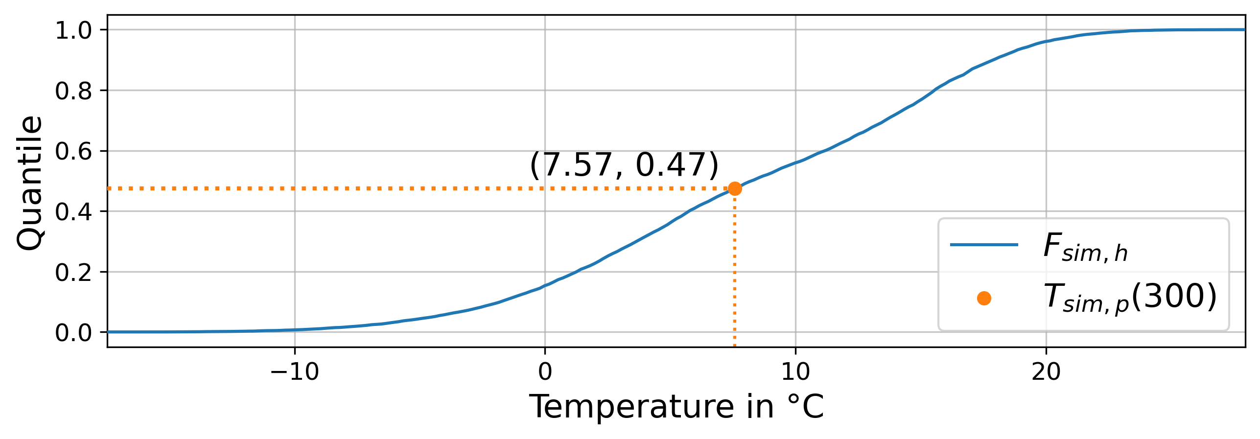
The additive quantile mapping procedure consists of inserting the value to
be adjusted (\(X_{sim,p}(i)\)) into the cumulative distribution function
of the modeled data of the control period (\(F_{sim,h}\)). This
determines, in which quantile the value to be adjusted can be found in the
modeled data of the control period The following images show this by using
\(T\) for temperatures.
Fig 1: Inserting \(X_{sim,p}(i)\) into \(F_{sim,h}\) to
determine the quantile value
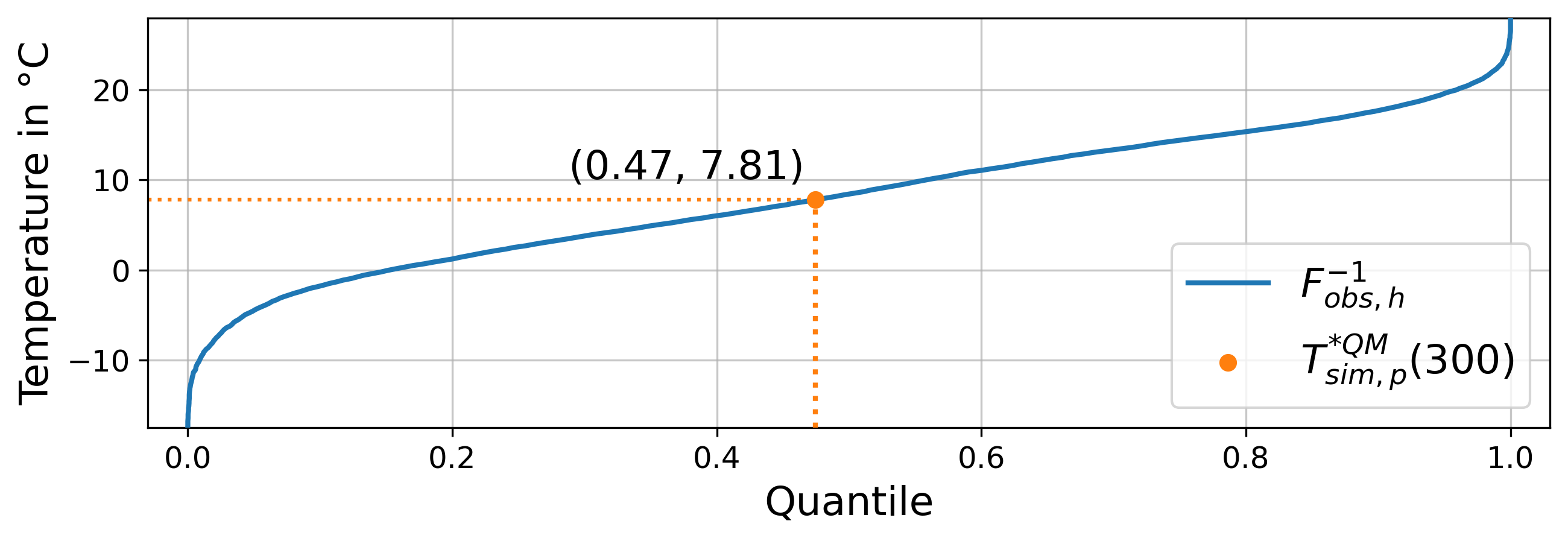
This value, which of course lies between 0 and 1, is subsequently inserted
into the inverse cumulative distribution function of the reference data of
the control period to determine the bias-corrected value at time step
\(i\).
Fig 1: Inserting the quantile value into \(F^{-1}_{obs,h}\) to determine the bias-corrected value for time step \(i\)
Multiplicative:
The formula is the same as for the additive variant, but the values are
bound to the lower level of zero.
Example:
The following example shows how to apply the multiplicative quantile mapping
technique on a 3-dimensional data set containing the variable “pr” (i.e.,
precipitation).
1BiasAdjustCXX\2--refinput_data/observations.nc\ # observations/reference time series of the control period3--contrinput_data/control.nc\ # simulated time series of the control period4--sceninput_data/scenario.nc\ # time series to adjust5--outputquantile_mapping_result.nc\ # output file6--methodquantile_mapping\ # adjustment method7--kind"*"\ # kind of adjustment8--variablepr# variable to adjust
The Quantile Delta Mapping bias correction technique can be used to minimize
distributional biases between modeled and observed time-series climate data. Its
interval-independent behaviour ensures that the whole time series is taken into
account to redistribute its values, based on the distributions of the modeled
and observed/reference data of the control period. In contrast to the regular
Quantile Mapping the Quantile Delta Mapping also takes the change between the
modeled data of the control and scenario period into account.
The Quantile Delta Mapping technique implemented here is based on the equations
by Tong et al. (2021)“Bias correction of temperature and precipitation over
China for RCM simulations using the QM and QDM methods”. In the following the
formulas of the additive and multiplicative variant are shown.
Additive:
(1.1) In the first step the quantile value of the time step \(i\) to adjust is stored in
\(\varepsilon(i)\).
(1.2) The bias corrected value at time step \(i\) is now determined
by inserting the quantile value into the inverse cumulative distribution
function of the reference data of the control period. This results in a bias
corrected value for time step \(i\) but still without taking the change
in modeled data into account.
The first two steps of the multiplicative Quantile Delta Mapping bias
correction technique are the same as for the additive variant.
(2.3) The \(\Delta(i)\) in the multiplicative Quantile Delta Mapping
is calculated like the additive variant, but using the relative than the
absolute change.
The following example shows how to apply the additive quantile delta mapping
technique on a 3-dimensional data set containing the variable “tas” (i.e.,
temperatures).
1BiasAdjustCXX\2--refinput_data/observations.nc\ # observations/reference time series of the control period3--contrinput_data/control.nc\ # simulated time series of the control period4--sceninput_data/scenario.nc\ # time series to adjust5--outputquantile_delta_mapping_result.nc\ # output file6--methodquantile_delta_mapping\ # adjustment method7--kind"+"\ # kind of adjustment8--variabletas# variable to adjust